1. Show the comparisons the naive string matcher makes for the pattern $abacab$ in the text $abacaabadcabacab$.

Solution: 27 comparisons

2. Show the comparisons the KMP string matcher makes for the pattern $abacab$ in the text $abacaabadcabacab$.

Solution: 19 comparisons

3. Show the comparisons the Boyer-Moore string matcher makes for the pattern $abacab$ in the text $abacaabadcabacab$.

Solution: 15 comparisons

4. Give a dynamic-programming solution to the 0-1 knapsack problem that runs in $O(nW)$ time, where $n$ is the number of items and $W$ is the maximum weight of items that the thief can put in the knapsack. Is the dynamic-programming algorithm a polynomial-time algorithm? Explain your answer.

Solution:

def zero_one_knapsack(v, w, W):
    n = len(v)
    dp = [0] * (W + 1)
    for i in range(n):
        for j in range(W, w[i] - 1, -1):
            dp[j] = max(dp[j], dp[j - w[i]] + v[i])
    return dp[W]

The algorithm above runs in $O(nW)$ time. Since $W$ is not a polynomial in the input size, the algorithm is not a polynomial-time algorithm. The algorithm is pseudo-polynomial-time algorithm.

5. Show that if $\text{HAM-CYCLE} \in P$, then the problem of listing the vertices of a hamiltonian cycle, in order, is polynomial-time solvable.

Solution: For every vertex $u \in V$, let $E_u$ be the set of edges that connects to $u$, enumerate two edges $e_1, e_2 \in E_u$ until $\text{HAM-CYCLE}(\langle G’ = (V, (E - E_u) \cup { e_1, e_2} ) \rangle)$ returns true. If $\text{HAM-CYCLE}(\langle G’ = (V, (E - E_u) \cup { e_1, e_2} ) \rangle)$ returns true, then we keep only these two edges and remove the other edges in $E_u$. After removing the edges, we can get the order by running a DFS from any vertex.

6. Show that the problem of determining the satisfiability of boolean formulas in disjunctive normal form is polynomial-time solvable.

Solution: The formula in disjunctive normal form evaluates to 1 if any of the clauses in it could be evaluated to 1. A cluase could be evaluated to 1 if there isn’t a literal $x$ that both $x$ and $\neg x$ appeared in the clause. Thus suppose there are $n$ clauses and the maximum number of literals in one clause is $m$, the time complexity is $O(nm^2)$.

7. Let $\text{2-CNF-SAT}$ be the set of satisfiable boolean formulas in $\text{CNF}$ with exactly $2$ literals per clause. Show that $\text{2-CNF-SAT} \in P$. Make your algorithm as efficient as possible. ($\textit{Hint:}$ Observe that $x \vee y$ is equivalent to $\neg x \to y$. Reduce $\text{2-CNF-SAT}$ to an efficiently solvable problem on a directed graph.)

Solution: To solve \text{2-CNF-SAT} in polynomial time, first construct an implication graph where each clause $(x \vee y)$ is represented by the edges $\neg x \to y$ and $\neg y \to x$. Then, find the strongly connected components (SCCs) of this graph using a polynomial-time algorithm. Finally, check for any variable $x$ such that both $x$ are $\neg x$ are in the same SCC; if none exist, the formula is satisfiable, otherwise, it is unsatisfiable.

8. Show how in polynomial time we can transform one instance of the traveling-salesman problem into another instance whose cost function satisfies the triangle inequality. The two instances must have the same set of optimal tours. Explain why such a polynomial-time transformation does not contradict the following theorem, assuming that $\text P \ne \text{NP}$.

Theorem: If $\text P \ne \text{NP}$, then for any constant $\rho \ge 1$, there is no polynomial-time approximation algorithm with approximation ratio $\rho$ for the general traveling-salesperson problem.

Solution: Let $I$ be an instance of the general TSP given a graph $G = (V, E)$ with edge costs $c(e)$. We construct a new instance $I’$ by constructing a graph $G’ = (V, E’)$ with edge costs $c’(e) = c(e) + \max_{e \in E} c(e)$. To see that $I’$ satisfies triangle inequality notice that for any three vertices $u, v, w \in V$, we have $c’(u, w) + m \le m + m \le (c(u, v) + m) + (c(v, w) + m) = c’(u, v) + c’(v, w)$, where $m = \max_{e \in E} c(e)$.

The optimal tours of $I$ and $I’$ are the same because the cost of the optimal tour in $I’$ is the same as the cost $C$ of the optimal tour in $I$ plus $nm$. Suppose that there is a tour $T’$ in $I’$ with cost $C’ < C + nm$. But then the cost of $T’$ in $I$ would be $C’ - nm < C$, which contradicts the optimality of $T$ in $I$. Therefore $T$ is the optimal tour in $I’$ as well.

Similarly we argue that every otpimal tour for $I’$ is an optimal tour for $I$. So let $T’$ be an optimal tour for $I’$ that has cost $C’$. Then cost of $T’$ in $I$ is $C’ - nm$. Suppose that there is a tour $T$ in $I$ with cost $C < C’ - nm$. But then the cost of $T$ in $I’$ would be $C + nm < C’$, which contradicts the optimality of $T’$ in $I’$. Therefore $T’$ is the optimal tour in $I$ as well.

The above polynomial time transformation does not contradict the theorem because the transformation does not provide an approximation algorithm for the general TSP. Let $I$ be an instance of the general TSP and let $I’$ be the transformed instance.

Using a factor 2 polynomial time approximation algorithm for $I’$, we obtain a tour $T’$ of cost $C’$ with the guarantee that $C’ \le 2OPT(I’)$. However, the cost of $T’$ in $I$ is $C = C’ - nm$. We may thus write $C \le 2OPT(I’) - nm = 2 (OPT(I) + nm) - nm$, or $C \le 2OPT(I) + nm$, which does not constitute a factor 2 approximation guarantee.

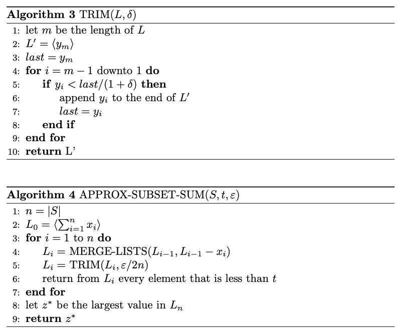
9. How can you modify the approximation scheme used in $\text{APPROX-SUBSET-SUM}$ to find a good approximation to the smallest value not less than $t$ that is a sum of some subset of the given input list?

Solution:

We’ll rewrite the relevant algorithms for finding the smallest value, modifying both $\text{TRIM}$ and $\text{APPROX-SUBSET-SUM}$. The analysis is the same as that for finding a largest sum which doesn’t exceed $t$, but with inequalities reversed. Also note that in $\text{TRIM}$, we guarantee instead that for each $y$ removed, there exists $z$ which remains on the list such that $y \le z \le y(1 + \delta)$.

10. Modify the $\text{APPROX-SUBSET-SUM}$ procedure to also return the subset of $S$ that sums to the value $z^*$.

Solution:

We can modify the procedure $\text{APPROX-SUBSET-SUM}$ to actually report the subset corresponding to each sum by giving each entry in our $L_i$ lists a piece of satellite data which is a list the elements that add up to the given number sitting in $L_i$. Even if we do a stupid representation of the sets of elements, we will still have that the runtime of this modified procedure only takes additional time by a factor of the size of the original set, and so will still be polynomial. Since the actual selection of the sum that is our approximate best is unchanged by doing this, all of the work spent in the chapter to prove correctness of the approximation scheme still holds. Each time that we put an element into $L_i$, it could of been copied directly from $L_{i−1}$, in which case we copy the satellite data as well. The only other possibility is that it is xi plus an entry in $L_{i−1}$, in which case, we add $x_i$ to a copy of the satellite data from $L_{i−1}$ to make our new set of elements to associate with the element in $L_i$.